Transcription and Analysis Tools

            Before writing your own programs, it is important to know what can be done with software that is widely available, and even free in some cases. In this part of the course we will survey what can be accomplished with several transcription and analysis tools. These include the programs SoundScriber, Elan, Toolbox and Excel.

SoundScriber

            SoundScriber is a program for transcribing digitized sound and video files and is available for free under the GNU General Public License. It includes normal playback features (e.g., Play, FF, Rew, Pause) as well as features designed specifically for transcription. The transcription features include keystrokes to control the program while working in a word processing window, variable speed playback, and “walking.” The walking feature plays a small stretch of the file several times, then advances to a new stretch with a slight overlap. With SoundScriber, it is possible to transcribe continuously without having to pause or rewind the recording.

            SoundScriber was a major advance in transcription tools in its day, but is now limited by advances in digital technology. These advances include changes in recording formats that SoundScriber is not equipped to handle. One major limitation of the program is that it cannot create a link between the transcription and the recording. Nevertheless, SoundScriber remains an easy to use, off the shelf solution to transcription needs.

ELAN

            ELAN is a transcription program available through the Max Planck Institute for Psycholinguistics. ELAN allows users to add an unlimited number of annotations to audio and/or video transcriptions. The annotations are synchronized with the recording. The annotations can take the form of a sentence, a gloss, or an observation about specific events in the recording. Annotations can be created in multiple tiers, which can be hierarchically interconnected. An annotation can either be time-aligned to the recording or it can refer to other existing annotations. The annotations can be printed in various formats and transferred to other programs.

            ELAN is a more sophisticated transcription program than SoundScriber, but its added features come with significant drawbacks. Each annotation has to be placed on the tiers manually. While this makes it possible to link the transcription to the recording, it is also a very time consuming process and makes continuous transcription impossible. Each annotation must be saved separately, which adds significantly to the time needed for transcription.

Toolbox

            Toolbox is a data management and analysis program available through the Summer Institute of Linguistics. The program is useful for organizing lexical data, and for parsing and interlinearizing texts. The Toolbox database management system allows customized sorting, multiple views of the same database, and filtering to display subsets of a database. The same database can include any number of scripts. Each script can have its own font and sort order. Toolbox includes a morphological parser that can handle almost all types of morphophonemic processes. It has a word formula component that allows users to describe the different affix patterns that occur in words. It has a user-definable interlinear text generation system which uses the morphological parser and lexicon to generate annotated text. Toolbox has export capabilities that can be used to produce a publishable dictionary from a dictionary database.

            The Toolbox site includes a lot of information on using the program, including the Toolbox Self-Training exercises. We will review the Toolbox Basics very quickly before doing an exercise on Interlinear Text which begins on p. 59 of the self-training manual.

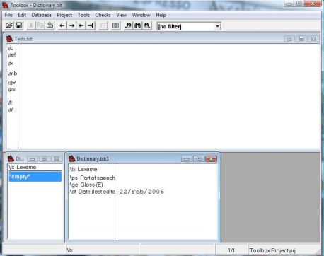
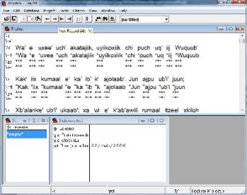
            When you install Toolbox on your computer, the Toolbox folder is placed in the Programs folder. This folder contains a ‘Start New Project’ icon. Double click on this icon to begin a new project. Toolbox will ask where you want to install your project folder and place a Toolbox Project icon on the desktop of the computer. Clicking on this icon will open the Toolbox window shown below:

The top half of this window provides the workspace for the text we will analyze. The bottom windows provide information that has been entered for each morpheme in the text. Since we have not entered any words yet, the windows at the bottom are empty.

            Down the left side of the top window is a list of Toolbox codes (called “markers”). The markers are the codes that Toolbox uses to keep track of the information in its database. We will analyze a text, which we will paste into the \tx (text) field of the window. The large white space in the top window can be edited like any word processing program. You can copy and paste a text document directly into this window on any of the fields with a marker. We will paste a text into the field with the \tx marker and paste a free translation of the text into the field with the \ft (free translation) marker. Toolbox will automatically link each clause in the text with a clause in the free translation so it is important to make sure that the clause divisions signaled by punctuation markers are consistent between the text and its translation.

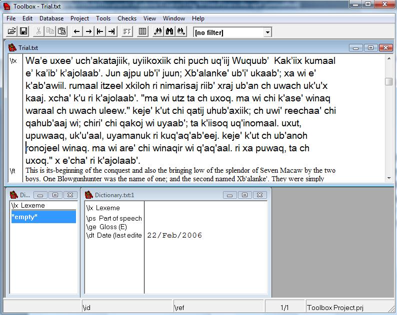
            I will provide a copy of the Popol Wuh, a K’iche’ Maya text. We will paste the K’iche’ text into the \tx field and the English translation into the \ft field. Toolbox does not accept a text with line breaks. An easy way to generate a text without line breaks is to paste the text into Word and then delete all line breaks. Once you eliminate the line breaks, you can paste the text from Word to the Toolbox fields. The result of this process is shown below.

            Toolbox is designed to perform many chores automatically which makes it very useful. One chore that the program can not perform by itself is finding the divisions between words and morphemes. Toolbox starts with a default alphabet which works well for English, but does not extend to languages with special characters, especially if they contain digraphs with two characters. Before inserting text into the program, it helps to tell Toolbox what characters will be used. Putting the cursor over the field markers and right clicking opens the Marker Properties window shown below.

            The Marker Properties window has a ‘Language Properties’ tab on the right side. Click on this tab to open the ‘Language Encoding Properties’ window. This window has tabs that allow you to Add, Copy or Modify the Alphabetical Order. Click the Modify tab to open the ‘Sort Order Properties’ window shown below.

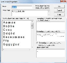This window shows the characters that Toolbox will use to process the text in the alphabetical order that will be used to produce a dictionary. The default character set does not contain any digraphs, in particular, the character set lacks any ejective consonants. You can add new characters by using the enter key to insert a new line, and then typing in any characters you wish to add. Characters are separated by a space. Edit the character set by adding the Mayan characters /B’, b’, Ch, ch, Ch’, ch’, T’, t’, Tz, tz, Tz’, tz’, K’, k’, Q’, q’/. Click the Ok tab when you have finished.

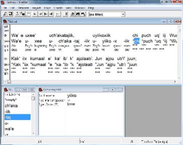
            We are now ready to begin analyzing the text. Ideally, we will add an English for each K’iche’ morpheme in the text. Since we probably don’t know how to gloss every K’iche’ morpheme at this stage we will focus on glossing the morphemes that we recognize. Toolbox allows you to add glosses selectively, so it is not necessary to gloss every morpheme. Go to the ‘Tools’ tab at the top of the window and click ‘Interlinearize’. This action adds two additional fields to each line of text. The \ge field provides space for an English gloss, while the \ps field provides a place for a part of speech label. The result of interlinearizing the text will resemble the following window.

The text in the top window can be edited directly. Entire words or parts of words can be selected for glossing. Select a morpheme with your mouse and right click the mouse. This action will take you to a window that asks if you wish to insert the morpheme into the dictionary. Clicking yes will add the morpheme to the lower window. Add an English gloss to the \ge field and a part of speech code to the \ps field. You can add hyphens to indicate that a morpheme is a prefix or suffix. I provide an example of the beginning of this process in the window below.

Excel

            Excel is Microsoft’s data management and analysis program. Excel has many features that are useful in linguistic analysis including a flexible entry system, sorting tools and a set of graphing tools. It is possible to set up an Excel sheet to perform different statistical tests. Excel also permits data to be imported from files generated by other programs. You can see the usefulness of these features in an analysis of sound production in five Mayan languages. The input data is the following:

            Yucatec           Ch'ol   Q'anjob'al        Mam   K'iche'

m        13        24        39        53        13

n          6          8          21        58        32

p          10        6          22        32        26

t          20        19        48        113      24

ch        10        18        46        88        29

k          9          8          32        100      38

j          2          14        16        47        13

l          18        8          18        54        29

w         10        7          28        38        23

I have not set up the data for the web to make it easier to import to excel. Excel allows the user to import data in various formats. One of the easiest formats is where each column is separated by a comma, tab or some other marker. You will need to copy these data from the web page and paste them to a notepad page. Be sure that each column is separated by a tab. Save your notepad as a text file named ‘sounds.’

            You can now import this data to excel by opening the excel program, clicking on the data tab, and then click on ‘Import External Data’ and ‘Import Data.’ A new window will open which will allow you to look for the ‘sounds’ file that you saved. Select the ‘sounds’ file and click Open. A new window opens and asks whether the data fields are separated by some character or have a fixed width. Since the data are delimited by tab stops in our file, we can simply click Next. A new window opens that should show the data arranged in columns. If the data is not arranged in regular columns go back to your original data file and make sure each data point is separated by a tab stop. If everything looks proper, click Next. This should bring you to step 3 of the import wizard. Everything should be ok at this point, and you should be able to click Finish. You could select a specific format for the columns at this point, for example changing the first column from the general format to the text format, but this isn’t necessary. You should now see a worksheet that looks like the following:

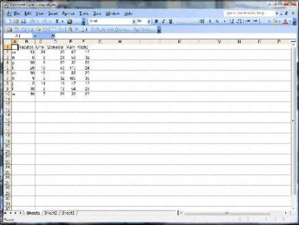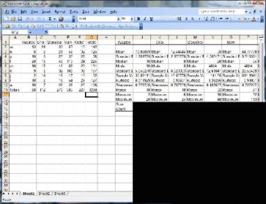
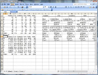
            It is obvious that the speakers of each language produced a different amount of speech, which affected the number of consonants the speakers produced. Excel’s analysis pack add-in allows users to extract a set of summary statistics that can show differences in the distribution of the consonant frequencies across the speakers. You can make this analysis by clicking on Tools, then Data Analysis, and final Descriptive Statistics. Clicking ok brings up a new window that asks you to specify the input range for the data you wish to analyze. You can select the columns under each language, including the first row with the name of the languages. Click on box that says Labels in First Row. Under Output Options, click the button Output Range and click inside the box. Next select a box to the right of the data table. You should see the cell name appear inside the box for the Output Range. Finally click the box for Summary statistics and click ok. A table of summary statistics should then appear to the right of your data table. This table includes the means, modes and standard deviations for the data.

            One question that we can ask of such data is whether the speakers of these languages use consonants with a statistically similar frequency of production. The chi-square statistic is a good statistical test of similarity since it automatically adjusts for differences in raw frequencies across subjects. One requirement for the chi-square test is that when the total number of responses is between 20 and 40, the test can only be used if all expected frequencies are greater than 5 (Siegel 1956). The chi-square test works by comparing the observed data against an expected measure based on the averages across the rows and columns. The first step is therefore to calculate the expected number of cases that correspond to each of the observations in the cells in the first table. Label the original table ‘Observed’ and the new table ‘Expected.’ The Expected table will have the same labels as the Observed table and will be the same size.

            The first step is to calculate the totals for each row and column as well as the grand total of the row totals. The result appears as follows.

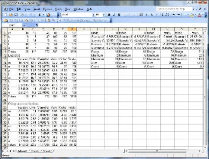
            To calculate the expected number for each observation start at the upper left cell for Yucatec. The observed frequency for /m/ in Yucatec is 13. The expected frequency of Yucatec is calculated by multiplying the total for /m/ (142) by the total for Yucatec (98) and dividing by the total number of observations (1290). The remaining expected frequencies can be filled in in the same manner. The resulting expected frequencies are shown in the following table.

            The final step is to compare the observed frequencies with the expected frequencies. If the difference between the two frequencies (observed - expected) is small, we can conclude that use of consonants is similar across the languages. The larger the difference, the more likely that the difference is statistically significant. You can use a table of chi-square statistics to calculate the statistical significance of this difference. The final step is to calculate these differences by squaring the difference between the observed and expected frequencies, and dividing the result by the expected frequency. The result for /m/ in Yucatec would be the square of its observed frequency (13) minus its expected frequency (10.7875969) with the result divided by the expected frequency. This calculation (13-10.7875969)*2/10.7875969 = 0.45374. This table is shown below. The total of the resulting rows or columns is the chi-square statistic, which is equal to 90.12 for the Mayan consonant data. This result is significant at the .01 level, indicating that we can reject the null hypothesis that speakers of these five languages use consonants with the same frequency distribution.

References

Siegel, Sidney. 1956. Nonparametric Statistics for the Behavioral Sciences. New York: McGraw-Hill.